
Become a member: Subscribe


NTS Headlines
Headlines by Category
Headlines by Year
- Money & Markets
- Weekly Solari Reports
- Cognitive Liberty
- Solari Builders
- Ask Catherine
- News Trends & Stories
- Equity Overview
- War For Bankocracy
- Digital Money, Digital Control
- State Leader Briefings
- Food
- Food for the Soul
- Future Science
- Health
- Metanoia
- Solutions
- Spiritual Science
- Wellness
- Building Weatlh
- Via Europa


Solari’s Building Wealth materials are organized to inspire and support your personal strategic and financial planning.


Building Wealth
This 6-pillar curriculum teaches the basic literacy we need to be personally and financially successful and to do so in a manner in which together we evolve a culture that supports the emergence of an advanced human civilization.


Missing Money
Articles and video discussions of the $21 Trillion dollars missing from the U.S. government

Connect with the wider network of like-minded Solari subscribers using our in-house social media platform, Solari Connect.


No posts
May 13, 2013 – Financial Perspectives
By Chuck Gibson
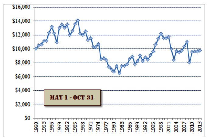
Since the calendar just turned its page to May I thought it good to visit that long standing Wall St. axiom regarding “Sell in May and go away (and live to see another day)”. For those not aware, it refers to the historically weak stock market during the periods of May through October and very strong performance for the remaining 6 months. I am not sure why it happens, there are lots of theories but it has been around for so long I think now it has become a self-fulfilling prophecy since it has so many followers. Regardless, this seasonality pattern really does have some very powerful statistical support. The charts below, courtesy of Breakpointtrades.com, show the data dating back to 1960 for the two time periods in question. Starting with $10k, if you invested the money at the start of May and pulled it out at the end of October every year, you cash pile would be slightly less than what you started with.
![]()
2 Comments
Comments are closed.

So I thought this was a pretty interesting concept and I ran a simulation against my own portfolio from 11/1/08 (after the crash) through 5/1/13. Even though my portfolio is pretty heavily weighted towards precious metals which have been slammed over the last two buying periods, (note: each stock was weighted equally in this simulation) the strategy still generated a 15.7% annualized gain after taxes (at capital gains rates). That is pretty impressive until I compared it to buy and hold over the same period which produced a 23.92% after tax gain. Kind of a rude awakening.
So as a reality check, I ran the Dow, S&P and Nasdaq indexes through the same model which produced a 7.84% annualized gain after taxes for the November to May strategy and a 15.98% return for the buy and hold method.
I don’t what data this guy is using or what he may be smoking, but I am not having any of it.
By Chuck Gibson
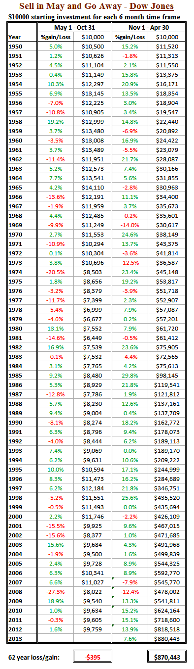
For clarity purposes since I did not do a good job framing the data in my post, the data presented was from 1950 to present on the DJIA index only. Therefore the outcome presented is for this dataset and this dataset only.
Any change to the framework of the dataset could, of course, make the results different. Therefore looking at any one specific year or any period other than that presented could yield different results. In addition to time frame changes, utilizing a different vehicle will most likely provide different results. Using gold, bonds, emerging market stocks or the Nasdaq for example, is highly likely to yield different results. I have not done any back testing to confirm or disprove therefore I cannot comment on the validity of its use.
Attached is a breakout of the yearly performance data which followed the framework stated above and clearly supports my blog post and is, for any person who deals only on statistical based facts, irrefutable. Clearly any change to the framework makes a different outcome statistically highly probable.
As a side issue and only because it was used to support of Mr Rea’s position and close out his discussion, I consider myself a reasonable person who is fully knowledgeable about the facts about smoking combined with two parents who died from smoking related illness I find the assertion of my use not germane to the discussion of a statistical based fact discussion.
See chart here.